The penalty in writing boolean arrays from lists to HDF5 via h5py is the conversion from list to Numpy array implicit in writing with h5py.
The order 10 ms h5py boolean list/array write time was not the issue, rather it was the synchronous reading of digital IO that was jamming up the system.
There is an officially-supported Windows-only Python NI-DAQmx module
and a community supported Linux + Windows Python NI-DAQmx module.
Both use Python ctypes to access the underlying C API and both require NI-DAQmx to be installed first.
Both are Python 3 compatible.
There are three NI-DAQmx download choices, pick one that suits your needs:
NI-DAQmx runtime (250 MB)
NI-DAQmx runtime + configuration (1.3 GB)
NI-DAQmx (1.9 GB)
Python NI-DAQmx: choose one of:
nidaqmx: official NI support, Windows only
pip install nidaqmx
PyDAQmx: support for Linux and Windows
pip install PyDAQmx
Python NI-DAQmx for Linux and Windows:
PyDAQmx
is the
community-supported
Python program for using NI-DAQ hardware from Python in Linux and Windows.
National Instruments provides Windows-onlycomplete Python API
via ctypes for NI-DAQmx.
The Python
nidaqmx_examples
are similar to those in LabVIEW, but with text based code.
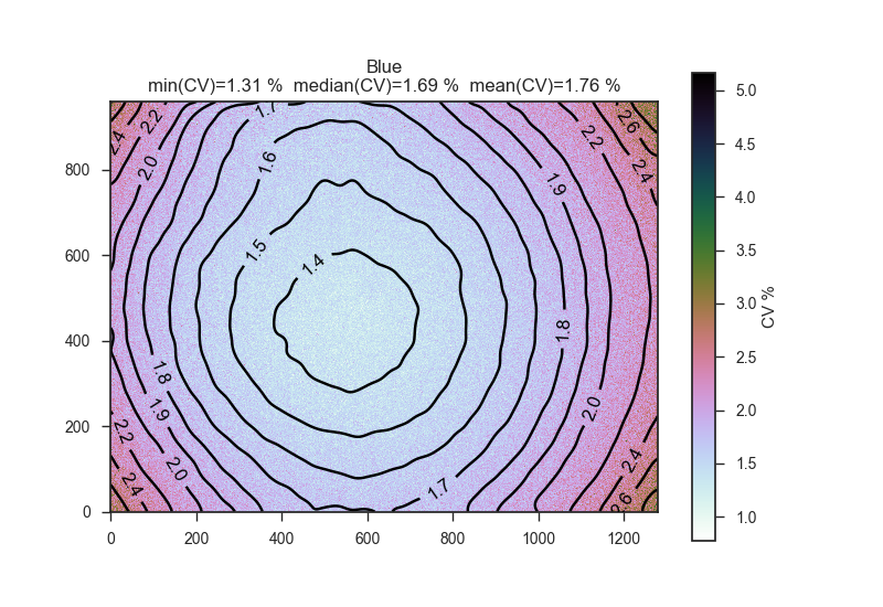
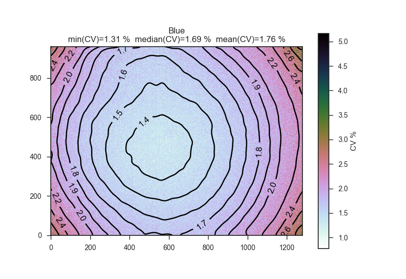
A first step in calibrating a whole-slide fluorescence cytometer is using a uranyl slide proving spatial uniformity to spatially normalize LED illumination and camera vignetting.
We then measure the coefficient of variation (CV) for each pixel, expecting the CV to increase away from the center of slide as in the following Blue and UV excited fluorescence images.
In this data, the estimated CV is over 50 images and 1.3 ms exposure.
The plots are created by
PlotCV.py.
coefficient of variation with UV excitation on uranyl glass.
fluorescent coefficient of variation with blue excitation on uranyl glass.
The next step is to test the system using fluorescent beads of known diameter, where the CV will be worse as a figure of merit vs. other systems.
The
coffee-can radar systems
have the advantage of operating at a 13 cm wavelength, so antennas are small and quite directional, relevant for clutter reduction and high spatial resolution.
Without external hardware, Red Pitaya output/input resides in the 0-50 MHz range.
Build a radar in this range with nothing more than two Red Pitayas and some dipole antennas.
The radar topology is using frequency translation via the second Red Pitaya acting as a bent-pipe transponder.
This is a high-tech, long-range version of
harmonic radar.
Particularly with software-defined-radio, it has become feasible for electronics enthusiasts and engineering students to build their own radar.
Here are a few projects.
WH2XBH licensed to MIT Lincoln Laboratory has a transmitter location of 42.624N, 71.486W which is at MIT Haystack Observatory near Westford, MA.
The licensed frequencies are useful for probing the ionosphere across a range of HF frequencies.
HF experimental licenses are in general not contiguous across the HF bands because of protected radio services such as government, aircraft, public utilities, and the like.
WH2XBH is licensed
at 1 Watt ERP with condition “the occupied bandwidth of the emission shall not extend beyond the band limits” for (approximately, see license for exact bounds):
Start freq [MHz]
Stop Freq [MHz]
2.0
2.17
2.19
2.49
2.51
2.85
3.16
3.4
3.5
4.0
4.15
4.65
4.75
4.99
5.01
5.45
5.73
6.2
6.77
8.35
8.37
8.81
9.04
9.99
10.1
11.17
11.4
11.6
12.1
13.2
13.41
14.99
15.1
17.9
18.03
19.68
19.8
19.99
20.01
21.92
22.0
23.2
23.35
24.99
25.01
25.55
25.67
30.0
ITU/FCC Emissions designator: generally the emissions are of type 500KW0W except where narrower.
The fifth letter refers to the modulation being sent.
fifth letter
modulation. Here, it’s W, which means any type of modulated or unmodulated transmission.
sixth letter
information content. Here, it’s 0, which means no inherently useful information is sent.
Modulation is sent, but it’s modulation useful for radiolocation, not for sending messages as a sole end goal.
seventh letter
information type. Here, it’s W, which means any type of information may be transmitted.
This might seem to conflict with the 6th letter, but what it actually means is any type of content, as long as information transmission is not the purpose of the transmission.
I can send jumbled up pictures or random numbers, but not broadcast a TV or music program.
This page is focused exclusively on United States of America Amateur Radio regulations.
Beacons in the Amateur Radio Service: for HF (sub-50 MHz) frequencies, 10-20 kHz bandwidth might be legally possible on these frequencies with up to 100 Watts conducted transmit power for one-way transmission under the Amateur Radio Service,
§ 97.305(c).
frequency range [MHz]
notional wavelength [m]
1.8 - 2.0
160
3.6 - 4.0
75
7.125 - 7.30
40
14.15 - 14.35
20
18.110 - 18.168
17
21.20 - 21.45
15
24.93 - 24.99
12
28.3 - 29.7
10
50.1 - 54.0
6
144.1 - 148
2
222 - 225
1.35
902 - 928
0.33
420 - 450
0.70
1240 - 1300
0.23
2300-2310, 2390-2450
0.13
Along with numerous higher frequency bands.
Note: 7.075 - 7.10 MHz is NOT phone/image in the lower 48 states of USA
Beacons may be locally or remotely controlled.
An easy method of legal remote beacon control may be accomplished via a simple website.
The control operator sees the status of the beacons and can click a button to turn individual beacons on/off from their smartphone without need for an app.
One control operator can control an unlimited number of stations remotely.
Legal Beacons under FCC Part 97 (Amateur Radio Service):
§ 97.203(g) beacon may transmit one-way communications
§ 97.203(c) beacon can transmit up to 100 Watts conducted power
§ 97.203(b) beacons may transmit on multiple amateur bands simultaneously, one “channel” per amateur band.
Examples of practical usage of beacons under § 97.203 include worldwide networks of beacons using a variety of emission modes exist throughout every amateur HF band.
The NCDXF network transmits 24/7/365 with 100 watts on several HF bands with stations worldwide since 1979.
§ 97.307(f)(2) No non-phone emission shall exceed the bandwidth of a communications quality phone emission of the same modulation type.
DSB-AM voice transmissions may perhaps occupy up to 20 kHz instantaneous bandwidth or so, although 10 kHz bandwidth is perhaps more common.
Perhaps we are transmitting an “image” or a digital “voice” transmission, in a manner that is convenient for ionospheric sensing with an HF radar beacon network.
Some people incorrectly latch onto § 97.203(d) which applies to automatic control beacons only.
That is, beacons that no human needs to actively monitor or control.
In contrast, we propose radar beacons that are remotely controllable over the internet via any web browser as has been well established.
Non-Beacon strategies relevant to VHF+ operations include:
Automatic control: No control operator, local or remote: § 97.113(d) Includes auxiliary, repeater, and space stations.
Test (> 51 MHz) Emissions containing no information: § 97.305(b) Test does not include pulse emissions with no information or modulation unless pulse emissions are also authorized in the frequency band. 1500 watts PEP conducted power limit, appears to be no bandwidth restriction.
Spread spectrum: § 97.313(j) Spread Spectrum (>222 MHz) May fill entire amateur band, 10 watts PEP transmit conducted power.
Most PCs made in the past decade are compatible with OpenGL, enabling extremely fast 2D and 3D animation–including from Python.
You DON’T have to learn OpenGL at all to make interesting 3-D plots from Numpy arrays.
VisPy
is a high-level easier to use OpenGL interface for Python, while Glumpy is a lower-level interface.