this will take several minutes without progress indicator e.g. 4000/10/60 = 6.6 minutes.
Type sync to be sure SD card is done writing.
Insert microSD card into Red Pitaya (contacts facing away from PCB)
Power up Red Pitaya with Micro USB jack nearest board edge.
The flashing LED settle down in 30 seconds to constant green and blue and double-flashing red (or, single flashing orange).
Accessing the Red Pitaya via web browser shows the graphical apps for oscilloscope, spectrum analyzer, and the App Store for free apps like SDR, VNA, etc.
You can also connect to the Red Pitaya via SSH or serial port console.
Connecting to Red Pitaya over Ethernet: the Red Pitaya uses Avahi so that you typically don’t have to search for its IP addresses.
The Avahi address is found as follows.
Use the last 6 characters of the MAC address on the Red Pitaya Ethernet jack (say 12:34:56), and on laptop web browser http://rp-123456.local.
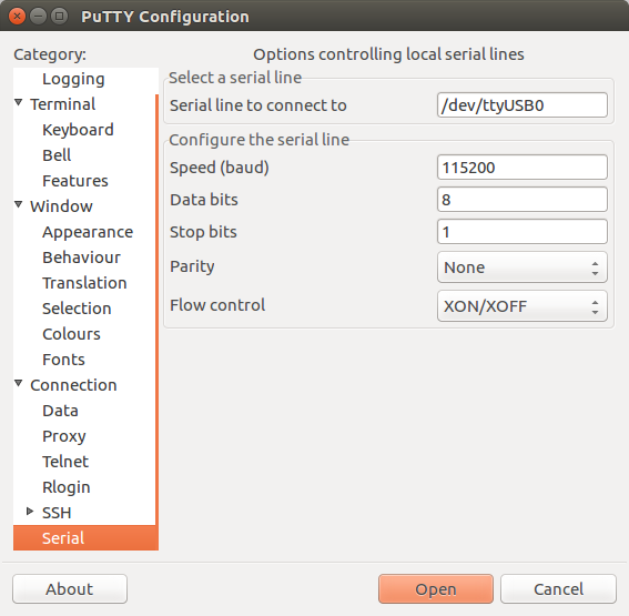
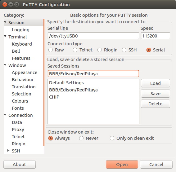
Serial port: if you can’t connect over Ethernet to Red Pitaya, you can plug a standard micro-USB cable from your PC to the Red Pitaya micro USB port next to the Ethernet jack.
Find the serial port
the Red Pitaya is on via
ls /dev/ttyUSB*
Probably it’s on /dev/ttyUSB0.
Then use
PuTTY
to connect to the Red Pitaya with the commonly used settings in these figures below:
PuTTY serial config for Red Pitaya
PuTTY serial config for Red Pitaya
For Pavel Demin’s ecosystem*.zip images for Red Pitaya ham radio, just extract the .zip file to the blank FAT32 formatted SD card.
The ecosystem*.zip contains numerous files and directories, unlike the single .img file in the procedure above.
Setup Red Pitaya HPSDR receiver image: format a micro SD card to FAT32.
Find the SD card device name from df – be sure you don’t overwrite your hard drive!
# Start the SDR Receiver compatible with HPSDR at boot timecat /opt/redpitaya/www/apps/sdr_receiver_hpsdr/sdr_receiver_hpsdr.bit >/dev/xdevcfg
source /opt/redpitaya/www/apps/sdr_receiver_hpsdr/start.sh
reboot the Red Pitaya
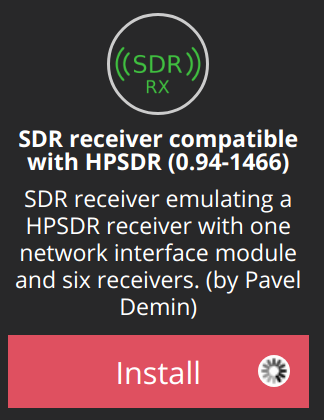
Install Pavel Demin six-receiver HPSDR from Red Pitaya marketplace.
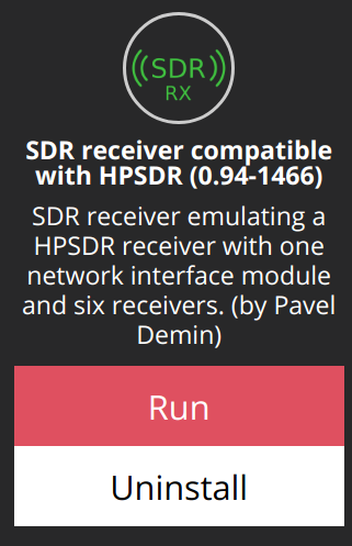
Run Pavel Demin six-receiver HPSDR from Red Pitaya marketplace (actually see step #6 to make HPSDR server autostart on boot).
Make a block diagram with GNU Radio Companion, using the hermesNB or hermesWB blocks.
If it doesn’t work, try
make uninstall
note that the version 1.2 of gr-hpsdr didn’t seem to update the connection between Gnu Radio Companion and the modules yet.
Use the top_block.py directly in Python e.g.
python top_block.py
It seems that GNU Radio ≥ 3.7.10 is needed as 3.7.9 just hangs waiting for connection.
If building GNU Radio, be sure to remove the system-installed gnuradio first.
apt remove gnuradio
If you get error
ImportError: libgnuradio-runtime-3.7.10.so.0.0.0: cannot open shared object file: No such file or directory
Ensure that /usr/local/lib is in LD_LIBRARY_PATH by in your ~/.profile adding the line
Normally we copy files over the network using encrypted SSH underneath SCP, SFTP or Rsync.
In the case of low power ARM CPUs, this may take an excessively long time since the low power CPU is overtaxed with encryption.
This method below is highly insecure, only for files you don’t mind sending unencrypted over isolated LAN only (don’t use this on any Internet-connected network!).
However it copies files over 10-100 times faster than SSH-based methods with low power ARM CPUs.
Note: You must have the port open in the firewall of the receiving PC.
On file-receiving PC, pick an open port in your firewall e.g. 60123, here we assume the receiving PC IP is 192.168.1.10
nc -l 60123 | tar xv
On Raspberry Pi, let’s say you want to recursively copy ~/myfiles to the receiving PC over the LAN
tar cfv - ~/myfiles | nc 192.168.1.10 60123
On both devices, you see a list of filenames as they’re copied.
Don’t forget to close the firewall port if you opened on on the receiving PC.
The
Semtech SX-1280
$3 three dollar ranging chip was
evaluated for LoRa ranging.
In general, 200 kHz RF bandwidth, 0.5 kbps data bandwidth and -130 dBm sensitivity trade lower speed for maximum range.
The narrow RF channel bandwidth helps range and reliability in the highly-congested 2.4 GHz band.
The Semtech SX-1280 2.4 GHz long-range radio transceiver in ranging mode may use 0.4, 0.8, or 1.6 MHz, relying on a subordinate unit to act as a sort of bent-pipe to relay the signal back with fixed device delay.
Without using more advanced techniques to constrain the problem, by
ΔR = c⁄2B
We would expect at best 3e8 / (2*1.6e6) = 94 meters range resolution.
Assuming a sensor fusion application, this ranging would not replace GPS in and of itself, but would indeed provide an excellent supplement for dense urban areas, such as large malls, warehouse/factory, and parking garages.
LTE location accuracy can do significantly better than this due to the typical 5-10 MHz or more bandwidth readily yielding sub-100 m location accuracy.
One of the key well-known limits of such low RF-bandwidth wireless location systems as demonstrated by SciVision, Inc. via model and simulation to US Dept. of Transportation personnel is multipath.
Multipath refers to the cancellations and self-interference causes from slightly time-delayed, strong reflections reaching the receiver.
Multipath is often worst in dense urban areas, likewise hindering accuracy of GPS.
CONOPS:
Exactly one LoRa ranging node can be ranged by the (likely infrastructure) controller at one time.
An ID number of 8 or more bits is used to uniquely identify nodes in range.
multiple controller stations improve accuracy (with cost of time)
Only the LoRa controller gets the ranging result (which is communicated to the node).
Pick an -np number suitable for your system (e.g. number of CPU cores)
If you also have Intel MPI installed, you might also want to try your program on OpenMPI for validation and sharing your program with a wider set of non-Intel MPI users.
Of course, you must compile your program with the appropriate MPI library.
Matlab / GNU Octave default axis scaling scales “x” and “y” axes proportionally to the axes values.
If one axis values span a much wider range than the other axis, the smaller span axis gets very thin and almost invisible.
Fix invisible axis in plot by axis('square') after imagesc()
rdat = rand(1000,10);imagesc(rdat)axis('square')
Axes representing actual data size has the axes to be representative of number of data elements (skinny images appear skinny)–insert axis('equal') after imagesc().
rdat = rand(1000,10);imagesc(rdat)axis('equal')
In Python Matplotlib, the same issue can be overcome with aspect='auto' property of ax.imshow().
Conversely allow the “true” axes ratio driven by the actual data aspect='equal'
Set this after the plot is created in axes ax by
importnumpyasnpimportmatplotlib.pyplotaspltrdat = np.random.rand(1000,10)
fg = plt.figure(layout='constrained')
ax = fg.gca()
ax.imshow(rdat)
# %% pick ONE of the following# non-shared axesax.set_aspect('equal','box')
# shared axes only (e.g. subplots(sharex=True))ax.set_aspect('equal','box-forced')
plt.show()
In July 2017, Bloomberg Radio in Boston moved from 1200 kHz AM to 1330 kHz WRCA-AM, and simultaneously enabled FM translator W291CZ-FM on 106.1 MHz.
The 255 meter elevation afforded by the 200 Clarendon building (former John Hancock building) in Back Bay gives a commanding view of the Boston area, just far enough from downtown so as not to be in the elevation null of the transmitting antenna.
In-building portable radio coverage of W291CZ to the west is remarkable, working well in the high-population business offices important to Bloomberg Radio.
Bloomberg 106.1 FM coverage Boston
WCOD interferes with W291CZ to the east and south of 200 Clarendon, including at least through Dorchester, WCOD covers up Bloomberg Radio so much that it’s unlistenable.
WCOD covers up Bloomberg in the vicinity of South Station, Back Bay, and so on until one block east of TD Garden, west of which the Bloomberg signal is OK.
The WRCA-AM broadcast originates 13 km from downtown Boston from the same tower complex and with similar power/antenna configuration as the former Bloomberg Radio broadcast from
WXKS-AM on 1200 kHz.
FM Translator co-channel interference can be considerable vs. legacy high-power FM stations.
Heading to the South Shore / Cape Code on I-93, after Exit 7 on I-93 onto MA-3, the
50 kW Cape Cod station WCOD
covers up Bloomberg on 106.1 FM.
FM translator permits for 106.1 FM have been issued for
Fitchburg, MA
and
Worcester, MA
further limiting DX coverage to the west and northwest.
The wide bandwidth of broadcast FM contributes to a very low capture ratio, so you’ll jump flip between music and talk radio without too much racket.
WRCA / WXKS-AM share a 5-tower transmitter plant.
FM Translators are useful to indirectly overcome AM interference.
Over the past 5 years that AM radio has become increasingly unusable even in suburban settings and hotel clock-radios are increasingly FM only.
Quality LED lighting interferes at least as much with AM radio as the compact fluorescent ballasts did.
The only time I can make serious use of AM radio from home is during power outages!
FM translator can be used to switch AM broadcast to all-digital.
Thus I welcome the 106.1 FM broadcast of Bloomberg Radio as an efficient use of spectrum.
An even more efficient use of the AM spectrum would be for the FCC to expedite all digital AM-band broadcasting, as in urban areas increasingly the AM stations are just used for their 60 dBu contour within which to place FM translator coverage.
Some of the first considerations for a harmonic radar application are discussed.
Maximum harmonic radar tag range: a 917 MHz radar using uncoded or pulsed CW may get about 10-15 meters range using 10 dBi antennas on the radar and 5 dBi passive tags.
Shifting up in frequency increases the gain, narrows directivity (beamwidth) of the antennas, yielding more angular selectivity for a given antenna size.
Active (powered) tags are required for extended ranges into 100+ meters standoff distance.
Many years of battery life are possible for such tags, and power harvesting methods and other modern semiconductor techniques may be applied to approach batteryless or battery-assisted tags for decadal service lifetimes.
Depending on the application (what you’re sensing) and the environment the tag is in, the tag could last from a month to a decade or more.
Tag lifetime is very system dependent.
This is a topic covered by patents and the open literature, including technology SciVision, Inc. has modeled and brought to fruition.
At a high-level, this is a key design parameter of the system.
Will classic angular selectivity (antenna beamwidth) be enough?
The 3 dB beamwidth might be > 60 degrees, and the 20 degree beamwidth (more important for discrimination) might be well in excess of 90 degrees.
Larger antennas, antenna arrays, or networks of radar antennas help increase angular/spatial target discrimination.
The classical multiplexing methods of TDMA, CDMA and FDMA may also be applied in various scenarios, particularly for active tags.
Active tags require a DC power source to bias the diode (or whatever semiconductor structure is chopping or otherwise frequency translating the input RF waveform).
This DC bias may well come from power harvesting or trapped charge FETs or the like.
Just a wee bit of bias gives a lot of signal gain (via reduced loss) thanks to the non-linear response of the diodic junction that creates the harmonics.
Passive tags inherently get their bias from the exciting RF waveform.
Intrinsic power harvesting, to abuse a term (much like how everything is AI/machine learning these days).
To predict performance of a harmonic radar requires a bit of knack and experience at RF systems performance.
You might engage with a consultant from SciVision, Inc., which has helped build valuations for several clients to impressive sums via custom model-based designs.
Likewise, unfeasible projects were shot down early by modeling and early prototyping.
The wavelengths in the general vicinity of LTE Band 26 & 5 (850 MHz cellular) are ideal for building penetration (phone indoors).
Akin to LTE bands 12,13 and 14 in the low bands (700 MHz), LTE band 26 at 806-861 MHz gives better long range coverage.
LTE carriers use carrier aggregation and at least LTE on the low-frequency (long-range) band as well as the high frequency band.
Clear WiMAX shutdown: LTE 2.5GHz Band 41 WiMAX termination drivers included 10x LTE spectral efficiency.
The need to pair high-frequency LTE Band 41 good for short range, high density use with band 26 good for suburban/rural is essential to modern mobile network operations.
Early WiMAX 4G adopters suffered coverage issues due to the simpler base station antennas of the time.
This was not the fault of WiMAX, rather it was because of the 2.5 GHz wavelength and free space loss.
Reasons to abandon Clear’s 2.5 GHz WiMAX may have included:
short wavelength no good for standalone carrier (best blended with longer wavelength bands for less dense areas)