GNU Radio FMCW radar USRP B200 and Red Pitaya
FMCW GNU Radio such as FMCW_usrp.grc setup is common to several IEEE articles. Do these setups actually work as shown? This general process is used for the PiRadar Red Pitaya radar code. The method extends to any short range radar using CW or FMCW modulation.
The signal processing algorithm must read/process the data in small segments. This is the only way to make a real time measurement. It conserves RAM/CPU for offline analysis as well.
Verify the data is read correctly–the raw data must make sense when plotted, or nothing else will work. Many software defined radios output complex single-precision floating point data. Often this data consists of 4 byte pairs of real/imaginary coefficients. Matlab can read such data with Matlab script for complex data as in read_complex_binary.m.

Incorrectly read FMCW sinusoid data--note very distorted waveform is NOT read correctly.

Correctly read FMCW sinusoid data--note clean sinusoid waveform, with at least two closely frequency-spaced sinusoids.
Slice FMCA data by chirp for processing. FMCW data and radar data in general is arranged into segments for each radar pulse/chirp so that you can estimate the covariance across FMCW chirps. This can be done by inspection since we’re only using a couple files to start. The chirp spacing is regular in number of samples–same throughout the entire file. For example, if the radar pulses at 10 Hz –> every 100 ms is a new measurement. When you’ve put these into a 2-D array, plot the data again to see the data is sliced correctly.
The 2-D array has each pulse/chirp data in a row, and the columns are sample number. Thus if I analyze 8 chirps each of 1024 samples, the array has shape 8 x 1024.
Estimate FMCW beat frequencies to get range. For FMCW radar, where the frequency sweep is linear, if target A gives a 1 Hz sinusoid and target B gives a 2 Hz sinusoid, target B is twice as far away as target A. Measuring absolute range starts with determining what zero range is in beat frequency. Just like real targets, the zero range (feedthrough) of the radar (which is the radar hearing its own transmission) shows up as a sinusoid. In general the radar hears itself as the lowest frequency sinusoid and also at the largest amplitude.
In a synchronized radar, this zero range feedthrough frequency (let’s call it F0) is constant for a particular radar configuration. F0 changes for each unique radar configuration (antennas, RF channel used, RF bandwidth used, etc.). In an unsynchronized radar such as the Red Pitaya currently is, F0 might change each time the same program is run, or even occasionally while the program is running. However the same problem occurs whether synchronized or unsynchronized (or measuring a jet engine)–one must first find F0. We measured with one of the Red Pitaya in FMCW radar mode that F0 stays constant for at least ~10 seconds at a time
Because F0 is so much larger in amplitude than any other sinusoid, you can do this with classic DFT (implemented via FFT) methods. These methods will find F0 approximately, with a few percent error. You will find F0 accurately with subspace estimation later.
To make the frequency estimation problem not consume an extremely large amount of RAM and CPU, we first reduce the problem as follows. If F0 is 100 kHz, but the maximum target frequency is 10 Hz, that is, we know that the only frequencies we’ll ever use are between 100,000-100,010 Hz, the problem because much easier to process if we first:
- frequency translate – multiply by complex sinusoid, this rotates the discrete-time samples in frequency, analogous to a shift register
- downsample – by anti-alias filtering and decimation e.g.
scipy.signal.decimate()
Thus instead of working with a file sampled at 4 MHz, we can downsample to 8 kHz, which conveniently you can play through your PC sound card if you want. When the target is not present, you hear a single tone, the F0 of the radar, plus low amplitude clutter. FMCW software defined radar processing: CWsubspace.py.
When the target is introduced near to the radar antenna, say 1-2 meters away, held still, not moving, you hear the F0 sinusoid apparently wavering in amplitude as that’s how closely frequency-spaced sinusoids behave–the amplitude envelope rapidly grows and shrinks for a tremolo effect like on the musical organs used at baseball games.
FFT-based methods exhaust RAM and CPU long before one can solve closely spaced sinusoid frequency estimation problems.
The family of subspace frequency estimation techniques include RootMUSIC and ESPRIT, implemented in
Python.
These Python subspace estimation functions such as ESPRIT are also callable from
Matlab.
These functions output estimated frequencies and the singular value sigma, which can be taken as a confidence measure of the estimate.
Informally, σ < 1 indicates low confidence–this estimate is suspect.
σ ≫ 1 indicates a high confidence, values in the tens or hundreds are possible in high SNR data.
Convert FMCW beat frequency to range using sigma as a qualifier, and that F0 is the lowest frequency, we convert target FMCW beat frequencies F_t to range R_t by:
R_t [meters] = c * F_t * T_m / (2*B)
Where c is speed of light, T_m is PRI i.e. time to sweep up or down in frequency, and B is the sweep bandwidth [Hz]. In general an FMCW radar measures F_t as F_t,measured = F_t,true + F0.
Unlike analog FMCW radars, software-defined radars must typically have a broad enough bandwidth to catch the entire chirp bandwidth. Unless for example one used an external VCO and the SDR can readily accept such, typical Ettus SDRs cannot quickly and deterministically change center frequency. At that point, you have simply a system more like the hardware-based radars, since you would be restricted to FMCW mode only for broad bandwidth. Instead, it is more desirable in general to have enough ADC/DAC bandwidth so that a chirp is synthesized within the ADC/DAC bandwidth and sent/received with SDR hardware VCO at a constant frequency.
With today’s SDRs, that limits chirp bandwidth to the 1-100 MHz range, maybe order 1 GHz with a high-end SDR. The FPGA or CPU has to be powerful enough to handle this streaming data rate–with a moderate PC and Ettus B200, you might get 5 MHz chirp bandwidth because you have to account for USB congestion and CPU utilization based on total TX + RX bandwidth. Of course, with RFNoC (if your SDR supports RFNoC) you can benefit greatly from processing directly on the FPGA.
Synchronize digital FMCW software-defined radar streams
Assuming the network/connection between the PC and SDR is stable, there should be a constant offset in number of samples between transmit and receive for a given radar configuration (e.g. sample rate, etc.).
Factors contributing to instability in terms of number of samples offset include: using virtual machine instead of directly running operating system, Wifi, congested Ethernet network, etc.
gr-radar has an approach to working around these issues by assuming the offset is at least constant for a particular run.
gr-radar computes the sample offsets for a run.
However, this OOT GNU Radio module is more oriented toward UHD Open Source driver, which is for Ettus Research SDR and other SDRs including Per Vices, Cubic SDR.
The Red Pitaya does not yet appear to implement UHD, but rather uses its own method of transferring streaming data PC ↔ hardware.
GNU Radio is oriented around streaming signals. In many forms of radar, one is oriented around pulsed signals. That is, one could get around the synchronization issues of streaming signals by getting the transmitter and receive cued up, and then starting both RX/TX together with deterministic FPGA delay. For many interesting radar systems there is more than one radar within range of targets and each other, so that a form of multiplexing channel access is necessary.
For FMCW, TDMA and FDMA are two popular radar multiplexing methods. For embedded radar system networks, where running on solar power, or where using small economical CPUs, streaming processing may be beyond the needs and/or budget. This leads one to a non-GNU Radio pathway, as Pavel has been exploring with a number of Red Pitaya configurations. Specifically, Pavel has provided a prototype radar Red Pitaya SD card image setup, such that individual pulses can be sent with the receive and transmitter synchronized.
GNU Radio gr-radar added the “Echotimer” self-calibration function in 2014.
Workaround these issues for non-USRP radars as mentioned in the first section.
Manual Synchronization test
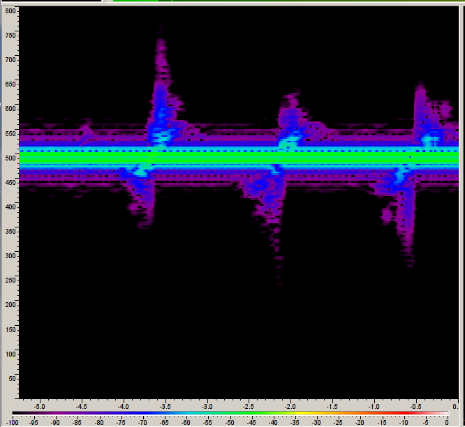
Spectrogram of 1 m/s moving target with USRP at 5.75 GHz, sweeping 1 MHz. Horizontal axis is time in seconds, vertical axis is frequency in Hz.
The moving 30x40 cm tinfoil piece was moved up and down from almost touching the radar antenna to about 1 m away. The main frequency displacement from the radar feedthrough was due to the Doppler shift. To reduce the signal processing burden, one can sweep over say 10 MHz if possible as this increases the tone separation.
The main point is to show that the USRP with plain GNU Radio FMCW was stable, even when restarting the program.
This spectrogram was created by:
- Ettus B200 with 5 cm piece of wire stuck in each of the TX/RX and RX2 ports for antennas
FMCW_usrp.grcsweeps from 5.750 GHz to 5.751 GHz, recording a 4Mbps complex float32 stream to disk of the beat frequencies. However, we know the beat frequencies will be very closely spaced (< 1 kHz) from feedthrough. This could be combined with next step if CPU can handle it. Obviously this would ideally be done on the FPGA.PlaybackFMCW.grcfilters and downsamples about the feedthrough frequency, where a 16 kbpscomplex64stream is more than enough for any possible beat frequencies. It writes a .wav file for convenience.FMCW_load_process_data.pytakes the .wav file, windows it, chopping out the bad interpulse data.- Using Goldwave or Audacity, listen to the wave file and get the live spectrogram.