Scientific Computing

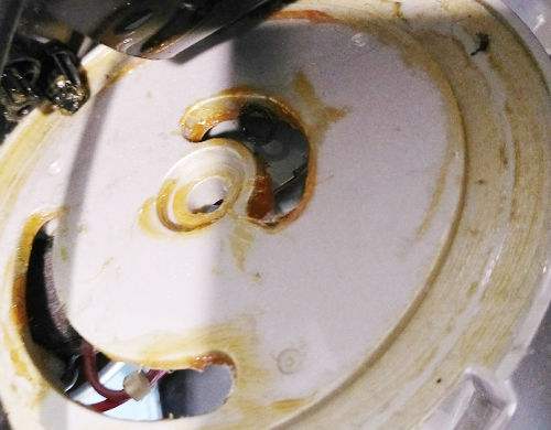
The Vornado Flippi fan series gets a number of bad reviews associated with short lifetime, some claiming days or weeks, prompting a return of the fan to the retailer. This Vornado Flippi V6 fan failed because a 120 Vac wire going from the fan base to the fan blade motor failed, possibly due to fatigue due to the oscillating motion of the fan head. This blue wire luckily was the neutral wire, and was of type AWM 1430 with VW-1 rating, 22 AWG. The wire manufacturer/model is Lee Yuen. The Flippi oscillating fan had an excessive amount of grease inside–not what one would expect from Vornado.

iFixit Vornado Flippi teardown

The Simpowel V8 Bluetooth stereo speaker costs less than $40, has been around for over 3 years (updated in 2016 to Bluetooth 4.0) and despite not having aptX, has adequate quality and sufficiently loud audio. Even in the stands of a baseball game, the Simpowel V8 is loud enough to hear the FM radio commentators for me and the person(s) sitting next to me, albeit set near maximum volume.

Key features of the Simpowel V8 Bluetooth speakers

• loud audio (baseball stadium tested)
• FM Radio
• micro SD card
• 3.5 mm input
• can run without battery installed
• battery is common and trivially replaceable
• multi-room Bluetooth coverage
• NFC “tap to pair” and “tap to disconnect”

Procedure based on Yocto Complete Image 3.5 with Linux laptop, using non-Arduino Intel Edison Mini Breakout board model EDI1BB.AL.K

Add your username to the appropriate groups on your laptop

adduser $(whoami) dialout
adduser $(whoami) plugdev

Logout and login on your laptop (reboot not required). On laptop:

dmesg

messages will stream to the laptop from Edison once it’s powered on.

Connect to Intel Edison via two microUSB Type B cables. Micro-USB type B are the common connectors everyone uses for phones etc.

Assuming Edison comes up on laptop as /dev/ttyUSB0 when both J16 and J3 are connected,

screen /dev/ttyUSB0 115200

Or use PuTTY.

Press Enter for login prompt. Login as root. There’s no password unless you set one previously.

See notes at bottom of this page for connection troubleshooting.

Software Update

It’s handy to be connected with PuTTY to the Edison, to see a much more detailed progress report.

Note this procedure erases everything on the Edison including data and configuration settings

On laptop, download latest Yocto Poky Complete Image. On laptop:

apt install dfu-util

Extract the Poky Complete Image, and from the extracted directory:

./flashall.sh

If you get a message

otaupdate.scr not found

upon Edison rebooting, the update is probably not going through. The process will take about five minutes (much longer than a normal reboot).

Confirm the proper version is uploaded by typing on Edison

cat /etc/version

201606061707

and at login you’d see with Yocto 3.5:

Poky (Yocto Project Reference Distro) 1.7.3

The Edison used space upon Yocto install was 76%. 319 MB free of 1.4 GB on a 2 GB Edison.

df -h

Intel Edison Configuration on first startup

from PuTTY window connected to Edison:

configure_edison --setup

Intel Edison Wifi can connect to WPA2 Enterprise as well as typical home WPA2 access points.

Unofficial Intel Edison Repository

On the Edison, add to /etc/opkg/base-feeds.conf

src/gz all http://repo.opkg.net/edison/repo/all
src/gz edison http://repo.opkg.net/edison/repo/edison
src/gz core2-32 http://repo.opkg.net/edison/repo/core2-32

Update repo cache

opkg update

The core2-32 opkg directory holds programs commonly used.

Troubleshooting

Both (two) green LEDs on the breakout board must be on and steady. If they are cycling on and off every several seconds, your USB port may not be providing enough power to J16. Maybe that USB cable is bad.

• Alternatively, the Edison eMMC flash memory could be corrupted, which requires reflashing

On laptop, unplug and plugin both USB cables, then type

dmesg

you should see

New USB device found, idVendor=8087, idProduct=0a99

FTDI USB Serial Device converter detected
Detected FT232RL
FTDI USB Serial Device converter now attached to ttyUSB0

If not, try being sure you are NOT plugged into a USB 3.0 port (has SS logo or blue colored inside). Try swapping cables at the Edison end–maybe one of them has the pins a little worn out. Poweroff and Power on your PC. Try another PC. If you don’t see these lines output by dmesg upon plugin, no other steps will work. You have to fix this first.

Type in your laptop

lsusb

you should see a line with

ID 0403:6001 Future Technology Devices International, Ltd FT232 USB-Serial (UART) IC

Type in your laptop

ls /dev/ttyUSB*

you should see

/dev/ttyUSB0

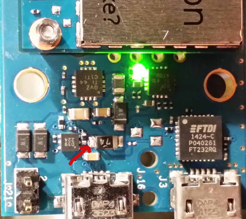
The red arrow points to the side of the “74” diode that comes right off the micro USB connector. With 5.00 volt input, downstream of the diode measured 4.72 V with the Edison idling. This voltage drop is expected due to the forward bias diode voltage drop.

Under 100% of one core CPU load measured 4.98 V on the USB side, and 4.66 V on the Edison side of this diode while powering from the USB port on the Verbatim 97928. The minuscule apparent 20mV voltage drop on the battery/USB side of the diode is likely to come from ohmic losses in the USB connector and cable.

Intel Edison alkaline battery life estimate is based on:

• Intel Edison measured power consumption
• assuming 2000 mAh for an AA battery

We estimate 10-12 hours of battery life on four AA alkaline batteries assuming continuous 100% CPU of one of the two CPU cores (other core idle). Normally the Edison will be mostly resting, drawing perhaps 100 mW.

Thus with mixed use, I might expect up to 4-5 days of continuous mixed use operation on 4xAA batteries for the Intel Edison.

Using a proprietary algorithm for static image analysis on images, and running the algorithm repeatedly,

the Intel Edison is about 2.35 times FASTER than the Raspberry Pi 1, using only ONE of the TWO Intel Edison cores.

The Intel Edison power draw was measured while using the Mini Breakout Board.

Yocto 3.0 has PulseAudio, BlueMan, XDG, etc. running in the background. This brings the idle current up 5 times as much as Yocto 2.1. To help preserve battery, perhaps disable unneeded services.

Yocto 3.5:

Yocto 3.0

Yocto 2.1

Benchmarks http://www.davidhunt.ie/raspberry-pi-beaglebone-black-intel-edison-benchmarked/ of Raspberry Pi vs. Beaglebone Black vs. Intel Edison.

The Intel Edison specifications show the idle power with Wifi as 35 mW, while we measure 88 mW. Lkely sources for “high” power reading are the two bright green LEDs on the USB adapter board, and the switching power conversion from 9 V to 1.8 V.

The Edison draws far less power at idle, perhaps 1/20 the power of the Raspberry Pi 3+ at idle.

The Raspberry Pi Zero W is a capable FTP/SSH server, but for field deployments, I would consider Compute Module 3 or Raspberry Pi 4.

This article is mainly about can be easily done with a Raspberry Pi Zero W vs. Compute Module 3.

Ranking key:

1. Cannot Install / Not working if Installed
2. Extremely slow, maybe single patient user only
3. slow, but perhaps usable for patient 1-3 users
4. adequate, may handle a handful of users (family, small club)
5. great, handles multiple concurrent users, not so much slower than a 10-year old Pentium 4 PC

Groupware (email/calendar) server

Citadel

Rank: 3

Citadel is an easy to install groupware server. Accessing features took a few seconds per click, and it didn’t seem that users would have the patience for Citadel on Raspberry Pi Zero.

FTP server

Rank: 4.5

Like SSH below, the Raspberry Pi Zero can handle a few connections at once, but is limited to less than raw Ethernet speeds due to:

1. CPU: USB-Ethernet onboard conversion
2. CPU: encryption (if using SSL/SSH, etc.)
3. CPU: filesystem – if using external HDD with FUSE (NTFS,exfat,etc.)
4. CPU: USB HDD – takes some CPU to manage the transfer from USB to external HDD
5. SD card: read/write speed

Web LAMP server

The Raspberry Pi as an NGINX or other lightweight server can work fine–test if your application might need the Compute Module 3 vs. Pi Zero.

Desktop workstation

Rank: 2 - 2.5

The Raspberry Pi 4 and Compute Module 3 are fast enough for light desktop use.

SSH server (port forwarding, SSHFS, remote management)

Rank: 4 - 4.5

The Raspberry Pi Zero W does quite adequately in this regard – you will feel just a bit of the CPU limitation when using many sessions or high Ethernet bandwidth.

FM transmitter

Rank: 4.5

The Raspberry Pi FM transmitter works splendidly – the program can be modified to transmit narrowband (~ 5kHz) FM on the 2 meter ham band, and for a wide variety of software defined radio tasks.

On the Intel Edison Arduino board, the J18 Arduino connector block TX/RX pins have the UART connected to /dev/ttyMFD1 in the default Yocto install.

The Mini-Breakout board Intel Edison has 1.8 V GPIO and can be damaged from connecting directly to 3.3 V or 5 V TTL logic. You need a level shifter board to do the interface to non-1.8V logic from the Mini-Breakout board.

To receive a stream from Intel Edison UART from a serial device that constantly streams output like a GPS NMEA stream.

At the Edison shell prompt:

stty -F /dev/ttyMFD1 9600
cat /dev/ttyMFD1

where 9600 is serial port device baudrate Text streams to console from UART serial device on Edison.

To two-way TX/RX from Intel Edison UART install:

opkg install screen

Connect interactively to UART device from the Edison shell

screen /dev/ttyMFD1 9600

where 9600 is serial port device baudrate

MRAA + PySerial make using the Intel Edison serial port easy from Python.

Install MRAA on the Edison and istall Pyserial:

python -m pip install pyserial

Verify serial port operation with:

import serial
import mraa

uart = mraa.Uart(0)

ser = serial.Serial(uart.getDevicePath(), 9600)

ser.write("TEST")
print ser.read(4)

Notes:

• Pyserial tutorial
• mraa UART from Python

Plug the USB-serial adapter into Intel Edison USB OTG host port. Check if new device is seen, from Edison terminal:

dmesg

If there isn’t a new assignment to /dev/ttyUSB*, the FTDI kernel module may be needed.

opkg install kernel-module-ftdi-sio

This assumes setup the Intel Edison opkg repository.

Verify USB-serial adapter in Edison terminal

dmesg

The reply should include

usb: FTDI USB Serial Device converter now attached to ttyUSB0

Update kernel if this doesn’t work.

Which Intel Edison Yocto version is installed?

configure_edison --version

Example: router with LAN IP address range 192.168.1.xxx.

The address discovery is faster if you know which port is open on your targeted device (host). However, you can also discover the device if open port is unknown.

Unknown open port scan:

nmap -sn 192.168.1.* --open

will tell you some of the IP addresses that are active on that subnet.

Options:

-sn

check if pingable (ping scan, not port scan)

--open

only tell which hosts appear to be up

Many devices will hide themselves from this scan, but it’s the first thing I try for finding a new device that attached to the network, such as an IoT device that isn’t trying to hide itself.

Port known, IP address scan: port scanning is much faster when the open port is known. Note in some rare cases, there is a firewall schedule or port knocking as additional security that could cause a port scan to fail.

Raspberry Pi port scan: assume known 192.168.1.xxx and that factory image has an SSH server on port 22.

Find the new Raspberry Pi IP address with

nmap -Pn -p 22 192.168.1.* --open

-Pn

nmap assumes each host is up

--open

only hosts with specified port open

non-nmap: scan IP address range with known open port: the pure Python program findssh.py, scans for servers with open ports in less than a second concurrently via Python asyncio.