Narrowband radar on lowband VHF 25-50 MHz
A radar based on Red Pitaya may operate for calibration or even primary purposes on lowband VHF (25-50 MHz). A primary reason one might use a radar on lowband VHF is for example measuring human, animal or vehicle targets using global license-free frequency bands. Such a radar can be handheld and battery powered, with collapsible antenna rods. The humanitarian demand for a such a radar could be significant as a much more compact and economical radar than the coffee can radars that have become popular after I developed the first such “personal radar” in 2006. There are global license-free frequencies in the 40-50 MHz range. One can consider the US license-free frequencies in the 40-50 MHz range.
For signal processing, using FFT-based methods breaks down for the narrowband radar because the frequency separation is too small. A common PC runs out of RAM, and certainly a small embedded CPU would as well. I tried to squeeze more frequency resolution out of the FFT, but a normal 8 GB laptop would run out of RAM, so it’s not workable on a 1 GB RAM Raspberry Pi 3. By instead using subspace estimation methods to find beat frequency CWsubspace.py the narrowband, small beat frequency separation seems initially possible in simulation. In initial measured data, the clipped ADC due to building 60 Hz pickup makes lots of extra fake beat frequencies. While working on the hardware fix to the clipped ADC (1:9 or 1:16 transformer for Red Pitaya input), one can make use of existing slightly clipping data by implementing a digital bandpass filter around the known center frequency. This is “fair” and standard practice, even without the clipping.
Signal subspace estimation techniques like ESPRIT and RootMUSIC find applications in radar, whether angle of arrival estimation or for close-spaced noisy sinusoid frequency estimation. There are bounds on subspace estimation performance as with any signal estimation technique, but in a subset of cases involving short range, narrowband radar, subspace estimators may have significant advantages. Subspace estimators give excellent performance vs. FFT for a given SNR, particularly with low SNR, with far lower RAM demands for a given accuracy vs. FFT. Mitigate CPU usage by using optimized signal subspace estimation FORTRAN code. Use a priori on number of sinusoids stronger than desired signal expected. Filter signal before estimation necessary as with FFT to constrain estimate to expected frequency range (e.g. automobiles not expected to drive 500 m/s)
Simulation
To parallelize the work of modeling and designing analysis, we can model expected beat frequencies for CW and/or FMCW. Simulate estimation with noisy sinusoids at the modeled beat frequencies. CW only gives Doppler. A model for beat frequency vs radial velocity is is piradar/CW_doppler.py as discussed here:
fbeat = 2 * v * ftx/(c-v)
FMCW can give range and velocity via the FMCW beat frequency. FMCW typically linearly sweeps the transmit frequency. Non-linearities in the sweep broaden the target uncertainty (increase error). A model for expected beat frequencies is in CalcBeat.py. FMCW beat frequencies in Hertz are defined by
f_beat= R * B/(T c)
where R is one-way range to target [meters], c is speed of light, T is chirp cadence [Hz].
- B = f_max - f_min
- chirp RF bandwidth
./CalcBeat.py -tm .1 -b 10e6For point target ranges [1, 10, 50] meters you may expect beat tones [‘0.7’, ‘6.7’, ‘33.4’] Hz. Using 10.0 MHz RF bandwidth, you may expect 15 meters range resolution by:
ΔR = c/(2 B)
If you sweep from 902..928 MHz, then B=26 MHz. However, using a priori knowledge about the targets, super-resolution techniques can enable better resolution proportional to SNR.
Performance
These plots demonstrate a system (CW or FMCW) that results in a true fbeat = 2.0 Hz. The estimation is performed by ESPRIT in piradar/CWsubspace.py
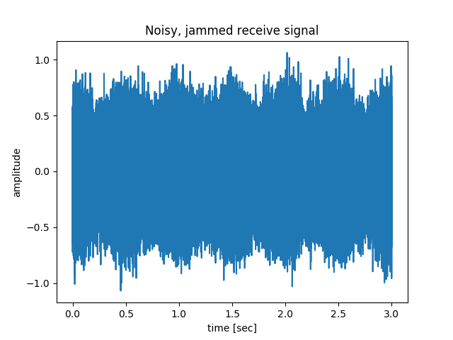
Noisy time domain received signal from CW radar. Dominant signal is carrier leakage as expected for non-nulled CW radar.
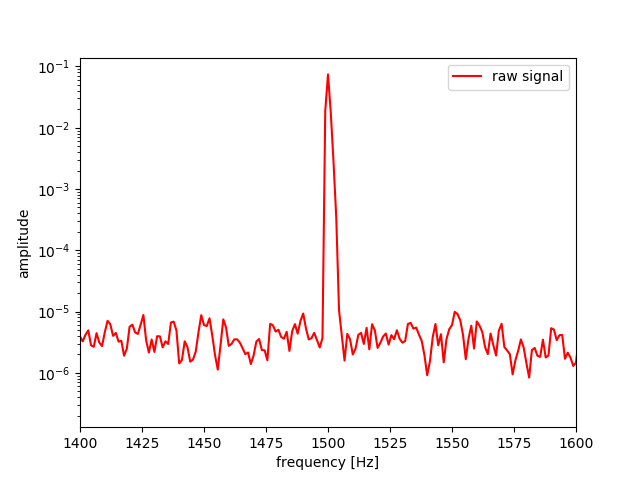
Frequency domain: receive signal is blurred together with CW carrier leakage--actual separation 2 Hz. FFT exhausts PC RAM without giving enough separation to resolve target beat frequency.
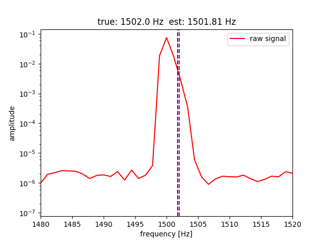
Frequency domain: receive signal is blurred together with CW carrier leakage--actual separation 2 Hz. Estimation error ~ 10%.
Estimation error with ESPRIT and block length 1000 gave beat frequency estimation error of order 10%.
This simulation from piradar/FMCW_sim.grc was conducted with GNU Radio and the standard built-in modules. The parameters were chosen for convenience of display in plots, not for a particular scenario.
| Parameter | Value | Units |
|---|---|---|
| sample rate | 1e6 | samples/sec |
| sweep freq | 50 | Hz |
| VCO modulation | ramp (sawtooth) | |
| sweep bandwidth | 100e3 | Hz |
The simulation was performed at baseband, so upon using DUC & DDC one could sweep from 40.7 to 40.8 MHz or whatever desired frequency.
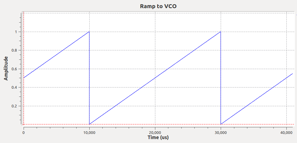
FMCW 50 Hz ramp input voltage to VCO.
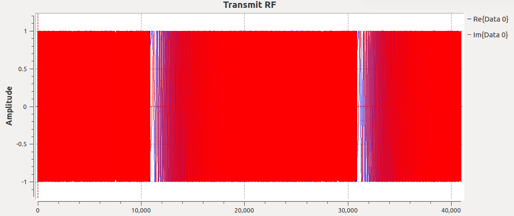
VCO output in time domain. Sweep starts at 0 Hz and goes to 100 kHz in baseband at 1 MHz sampling rate with 50 Hz cadence.
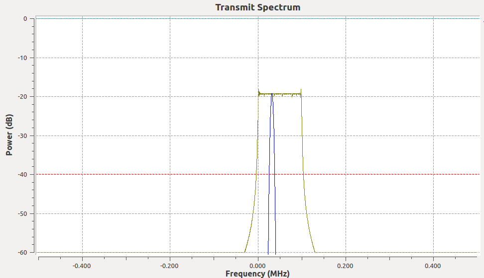
VCO output in frequency domain. Sweep starts at 0 Hz and goes to 100 kHz in baseband at 1 MHz sampling rate with 50 Hz cadence.
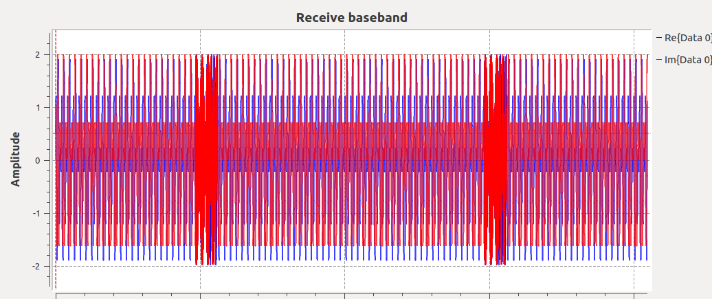
FMCW Demodulated output--pair of targets. Periodic glitches due to discontinuity at ramp reset.
The glitches are customarily eliminated in a straightforward way by dropping those samples (or skipping them) since they are inherently periodic.
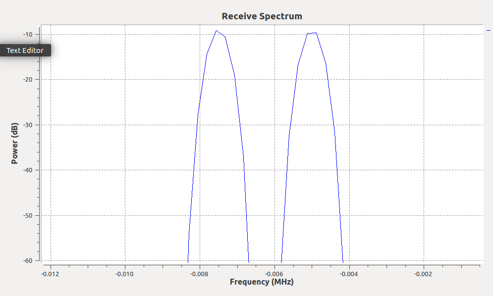
FMCW Demodulated output spectrum--pair of targets. Periodic glitches due to discontinuity at ramp reset.
The receive spectrum shows two distinct targets–one with a beat frequency of about 7 kHz and another at about 4.7 kHz. This corresponds to a range of about 210 km and 140 km – perhaps an F-region and E-region ionosphere radar return, respectively. The parameters used in these plots were more suitable for HF (2-10 MHz) measurements of the ionosphere.
Using low-band VHF, we can sweep a few MHz in the license-free bands, and sweep at a faster cadence. Let’s say the radar sweeps 5 MHz at a 1 kHz cadence, then a target 20 meters away returns a 667 Hz beat frequency.