Scientific Computing

Some Windows-oriented computers like Microsoft Surface with “Connected Standby” or “Modern Standby” may not be well supported in Suspend / Sleep with Linux yet. Consider having such a system lock on lid close until the Linux kernel is updated to support these newer power states. For better security in general, shut the laptop down while in transit in case of loss or theft. Locking screen with screen turned off gives sufficient power savings for short walks.

Force Linux lock on lid close with a systemd-based Linux distro such as Ubuntu by editing “/etc/systemd/logind.conf”, uncommenting line:

HandleLidSwitch=lock

Reboot the computer and verify lock behavior on lid close.

Reference:

• Microsoft description of traditional S3 standby vs. connected standby vs. modern standby
• Lock on lid close may not work when the laptop is physically docked, but does generally work when the laptop is out of dock. Do the manual lock if this doesn’t work when physically docked.

Intel Distribution for Python utilizes the conda package manager, set to the “intel” channel.

Pros: Intel Python uses highly accelerated math library versions of popular packages like Numpy, Scikit-learn, etc. reside.

Cons: Intel Python is slow to update to new library versions. Anaconda updates within a couple days, but Intel might take weeks or months to update the libraries.

Note that standard Anaconda Python already gives MKL performance in some libraries like Numpy and Scipy. We generally use the regular Anaconda instead of Intel Python to get updated libraries with most of them having MKL.

The convex hull is frequently used to process a pixel region. To find the indices of the outer edge of the convex hull may be accomplished using the distance transform. I do not claim this to be the most efficient method. This algorithm gives similar results to Matlab boundarymask().

Algorithm

By definition, the distance transform of all region edge pixels to the background is identically one. The chamfer distance transform is suitable for smooth regional boundaries, and has significant speed advantages over more brute force approaches that may be more generally applicable for non-smooth boundaries. Use either masked image arrays or use NaN as a sentinel value in 2-D array mask. SciPy ≥ 0.17 is assumed.

import scipy.ndimage as ndi

boundary_mask = ndi.distance_transform_cdt(~np.isnan(az), 'taxicab') == 1

For the smooth boundary cases I tried, distance_transform_cdt() was six times faster and gave equivalent results to the more general distance_transform_edt().

Notes

Reference

It’s a good idea to breakup project code into distinct subdirectories. It can be useful to have a CMakeLists.txt for each of these directories that are included from the top-level CMakeLists.txt.

Assume a C project with subdirectory io/ and top-level CMakeLists.txt:

project(benchmarks LANGUAGES C)
enable_testing()

add_subdirectory(io)

add_executable(benchIO bench.c)
target_link_libraries(benchIO PRIVATE iohdf)

and in io/CMakeLists.txt:

add_library(iohdf ...)

add_executable(testh5 testh5.c)
target_link_libraries(testh5 PRIVATE iohdf)

add_test(NAME h5io COMMAND testh5)

Build a little test script in io/ directory to test just HDF5 I/O, and compile the whole program from the top level directory, then test the main program and subdirectory libraries:

ctest --test-dir build -V

CMake Directory variables: to refer to the parent project directory use ${PROJECT_SOURCE_DIR}. If using nested projects, ${CMAKE_SOURCE_DIR} refers to the highest level CMakeLists.txt directory

Edit all CMakeLists.txt recursively: on Linux / Unix systems, edit all CMakeLists.txt in a project with a command like

gedit $(find -name CMakeLists.txt)

Related:

• Easy install Cmake
• Platform independent builds with CMake

Array broadcasting (no bsxfun() needed) is in Matlab and GNU Octave

Array broadcasting can minimize copying of large arrays in memory or excessive looping over arrays, both of which can be very inefficient. However, there are certain cases particularly with JIT compilers where looping can be faster than array broadcasting. Often the clean, clear code enabled by array broadcasting outweighs those edge-case possible gains. As always, make a simple benchmark if you’re concerned about a particular case (broadcast vs. loop) and for Python try Numba.

bsxfun is no longer needed for:

• plus
• minus
• times
• rdivide
• ldivide
• power

and many more operations.

If A has size 4x5 and B has shape 1x5, A .* B, A + B etc. just work without bsxfun(), provided the N-D array dimension multiplied is of matching shape.

This is important for clarity and conciseness of syntax. bsxfun() is a factor that drove me to using Python over Matlab almost entirely.

A .* B

can result in

error: operator *: nonconformant arguments (op1 is 5x4, op2 is 1x5)

Assuming A and B are compatibly shaped when transposed, try:

A .* B.'

Use .' to transpose because ' means take the Hermetian (complex conjugate) transpose. Remember that Matlab does memory copies (expensive for large arrays) on transpose. Python transposes are “free” O(1) since they’re just a view into the original array (pointer tricks).

Programs earlier than these versions did require bsxfun().

Fortran 95 brought function spread() for efficient array broadcasting by replicating the array in memory.

Python-based data analysis is dominating many fields. In astronomy and geoscience applications, Python dominance is increasing. Consider a widely valued language like Python inside of a niche, virtually unknown language outside a few specialties.

Installing Python for the first time: Miniconda Python is a 100 MB download–it won’t initially take several gigabytes of hard drive space like Matlab and IDL.

Package distribution can occur via a website or preferably, a centralized conda or pip repo. For example, to install popular data analysis modules:

conda install pandas scipy matplotlib spyder

IDL vs. Python syntax gives NumPy/Python equivalents to common IDL commands

IDL is a bit distinctive in its syntax. IDL and Matlab syntax remind me a bit of Fortran, while Python is C-based, including that Python has 0-based indexing and C-order array axes. Mayavi also gives advanced 3-D visualization.

Jupyter Notebook makes an IDE in your web browser, and you can make remarkable animated, interactive 3-D plots as well with Ipyvolume.

conda install jupyter
pip install ipyvolume

HDF5 can handle large and small datasets quickly and easily. Assume HDF5 file terabyte.h5 with double-precision float variable X of size 100000x2048x2048 (3.4 TB). Let’s load the first frame of the 2048x2048 image data, and write it variable first to image.h5. The with syntax uses Python’s context manager, which closes the file upon exiting the indented code section under with.

import h5py

with h5py.File('terabyte.h5') as f:
    img = f['X'][0,...]

with h5py.File('image.h5') as f:
    f['first'] = img

IDL supports Python

• call Python function from IDL
• IDL from Python.

Call GDL from Python: GDL Gnu Data Language is free open-source alternative to IDL, compatible with most IDL syntax.

from Python, call IDL/GDL functions by simply import GDL. See PYTHON.TXT

Call Matlab from Python and Python from Matlab:

• call Matlab function from Python
• call Python function from Matlab

Removing the left N columns from a text file can be done with the one-liner below. This example trims off the first 2 columns of each row of a text file “old.txt”, resaving as “new.txt”:

cut -c2- > new.txt < old.txt

For example, clean diff output of all the plus/minus signs or eliminate unwanted characters in the first column(s) of a text file.

Related: remove right columns from text file

Old Fortran or COBOL programs may have columns 73-80 filled with vestigial card sequence numbers. Trim rightmost columns as in this example. This keeps the first 72 columns of text from “ancient.for” on each row, resaving as “ancient.f”.

cut -c-72 > ancient.f < ancient.for

Any trailing whitespace (up to 72 characters for this example) remains.

Related: remove leftmost columns from text file

Wake-on-LAN can also work worldwide (over WAN Internet), in case a PC 10,000 km away gets turned off accidentally. To turn on a target PC from anywhere in the world, first setup the target PC and router port forwarding. For simplicity/clarity we assume the following arbitrary parameters, which will be unique for the target Linux PC:

• target interface: eth0
• target PC static LAN IP: 192.168.1.100
• target public WAN IP: 1.2.3.4
• public WoL port forward: 10009
• target MAC: 00:11:22:33:44:55

Remote Linux PC: modern Linux distros such as Ubuntu have WakeOnLan configured in NetworkManager.

1. Settings → Network and select the wired LAN interface to use for WakeOnLan.
2. under the “Ethernet” tab, seee that “Wake on Lan: Default” is checked. No Wake on LAN password is needed for most use caes.
3. copy down this “Device” hexadecimal string, this is the MAC address to turn on the PC remotely.

Confirm the correct MAC address by typing in Terminal

ip a

Have someone nearby it in case it doesn’t turn it back on–shutdown remote PC for testing.

On a laptop:

apt install wakeonlan

Wake PC on same LAN

on control PC, on the same LAN

wakeonlan 00:11:22:33:44:55

using the MAC address of the target PC of course.

If PC didn’t turn on, ensure BIOS/UEFI settings have Wake On Lan enabled. Try a discrete Intel Ethernet NIC, some motherboard NICs don’t work for Wake-on-LAN

setup worldwide Wake-on-LAN

To wake-on-LAN from anywhere in the world, using example parameters at top and after doing the procedure above, further do:

1. Router: port forward 10009 to 192.168.1.100 port 9
2. To use without Dynamic DNS service, have the PC auto-send email when the public IP address changes.

From the control PC on a different network type in Terminal:

wakeonlan -i 1.2.3.4 -p 10009 00:11:22:33:44:55

and target PC should power on.

Notes

• Ubuntu WoL setup
• Ubuntu TLP config
• notes

Legacy Linux remote PC setup

This procedure is for older Linux distros that don’t have WakeOnLan config in NetworkManager.

Install ethtool

apt install ethtool

Add the following line to /etc/network/interfaces under the interface to control auto eth0

up ethtool -s eth0 wol g

Edit /etc/init.d/halt, changing text near top to:

NETDOWN=no

instead of yes.

Edit/create /etc/default/tlp with line

WOL_DISABLE=N

Note link/ether for eth0–this is MAC address

ip a

Reboot target PC, then shutdown target PC for testing

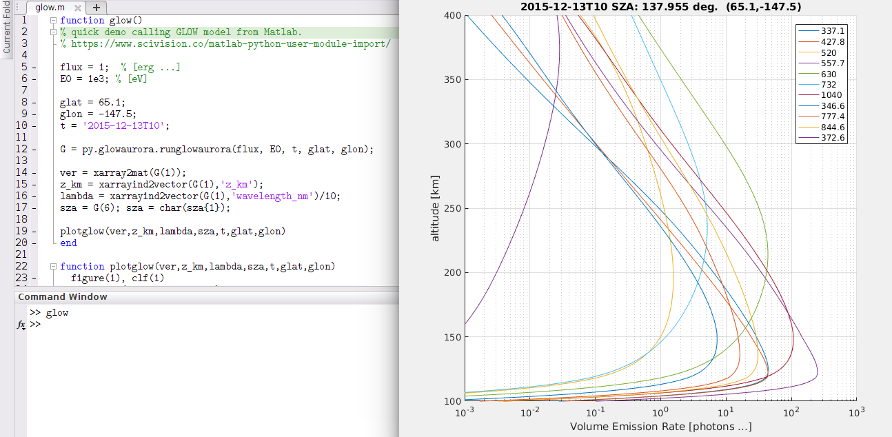
Stan Solomon and the NCAR team have greatly cleaned up GLOW auroral energy deposition and kinetics model. The new version number is 0.981, and since it’s mostly to Fortran 90/95 standards, it’s easier to use and modify, along with being more stable.

Updated GLOW Python/Matlab code is available for new GLOW 0.981.