baseband IQ data (not just speaker audio recording) for various HF radars.
baseband data from homodyne radars such as the many variants of tin-can radars out there.
The reason is that I find little if any such data publicly available.
It can be useful to get a preview of real data before building a hardware version, or as I recommend, configuring a software defined radar.
Motivations for using DSSS on an HF radar include:
great range and Doppler resolution.
LPI
not bothering other spectrum users (narrowband or wideband)
low peak power
readily doable with < $200 SDR
I can make up hypothetical waveforms as you like.
But some people will prefer to see real data
a) not interfering with PiRadar
b) PiRadar not being bothered by such data.
So again, I’m looking for data you’re willing to publicly release say via Zenodo (I can upload for you) so that radar students and engineers can have these waveforms to test coexistence.
Perhaps the simplest waveform a radar can use is a continuous unmodulated tone.
You will get no direct range measurements from such a system, but you will inherently get Doppler beat frequency fbeat measurements proportional to radar transmit frequency ftx for target radial velocity v using speed of light c.
From the program CW_doppler.py:
fbeat = 2 * v * ftx/(c-v)
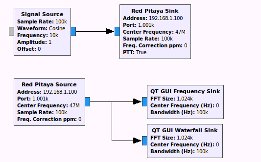
A software defined radar implementation of a CW Doppler radar using GNU Radio might look like this diagram:
CW Doppler Software Defined Radar using GNU Radio and Red Pitaya.
Avoid zero center frequency: IQ imbalance by the technique of moving the main transmit/receive frequency away from the center frequency of the complex baseband, to avoid interference from IQ imbalance.
Estimate radial velocity from CW software defined radar with unmodulated CW (pure everlasting sinewave emission, delta functional in frequency domain).
The estimation problem is accurately determining fbeat by which v is estimated.
Of course, the return signal is highly corrupted by noise, not least of which is the phase noise of the transmitter, particularly under 100 MHz where the Doppler shift is relatively small, compared to a 2.4 GHz radar.
A peak-finding algorithm on the frequency domain representation of the return signal obtained via FFT is typically not the best choice.
If noise is a problem, and you want to find multiple targets, subspace frequency estimation methods are known to be highly precise for solvable problems.
Subspace frequency estimation
code for Python, Fortran, C and C++.
Matlab’s implementation is very inefficient by comparison–Matlab takes far longer to solve and with poorer results.
Expected beat frequencies: the radar transmits at 47.010 MHz, and for vehicles on the highway, by the equation above, most return signals will be in the 47.0099 MHz to 47.0101 MHz range, that is, the beat frequencies will be less than 100 Hz magnitude and most less than 10 Hz magnitude.
The exact beat frequency for a given trajectory and fixed radar parameters depends entirely on the radial velocity.
Target true velocity estimation can be obtained from radial velocity.
This can be computed and used to invert measurements to get an estimate of true target velocity given oblique measurements.
The usual non-uniqueness issues apply.
Attempting to estimate bounds on range using unmodulated CW radar from targets with known travel paths and speeds can be a thought exercise, but not necessarily a fruitful pursuit.
It is more practical to apply frequency modulation, whether stepped or swept in frequency to enable traditional range measurements with fewer a priori constraints.
An example of
stepped frequency FSK CW radar paper.
We did a brief PiRadar transmission in the 80 meter ham band today and received on a second antenna.
We don’t have the system calibrated yet so we don’t have a quantification on what we were measuring.
Every radar needs calibration to get usable range, Doppler and other measurements.
Expanding upon section 3a of the PiRadar functionality test, we describe the materials needed to do an outdoor improvised radar range test.
This test can be run independently of the tests from Sections (1) and (2) that are about the radar timing.
The idea is to test the system in pieces so that it’s not too complicated testing everything at once.
The dipole antennas will be about 4 meters in length.
Thus several meters of coax cable between the dipole feedpoint and the Red Pitaya is required to avoid breaking the Red Pitaya SMA connectors.
The coax should come out perpendicular to the dipole for a few meters or else the radiation pattern gets goofed up.
Solder a 10Kohm resistor across the dipole feedpoint to dissipate static electricity buildup that can zap the Red Pitaya input.
Home Depot has 1.2 meter long wooden dowels for $1, one could connect 3 of them together and then let several centimeters of the solid wire stick past the ends.
There are cheap cables and connectors on eBay, however double-check that they aren’t RP-SMA (doesn’t mate with SMA) or that they’re overseas and take 30 days to ship.
Vector graphics in a PDF may be displayed directly in a webpage by using SVG.
SVG is widely supported by virutally any web browser without plugins.
This avoids having to download a PDF, while preserving full vector graphics resolution.
Before conducting a field test, it’s beneficial to test the constituent parts of the radar.
Since this is an HF radar, using a higher frequency where it’s easier to build antennas to test with targets smaller and closer than the ionosphere can be expedient.
In general the three essential functions of a radar are:
time synchronization: ability to send/receive with accurate absolute time–here provided by GPS into the GPIO and FPGA.
transmit: ability to send a signal at a desired RF frequency and bandwidth, with accurate timing
receive: ability to receive a signal at a desired RF frequency and bandwidth, with accurate timing
Transmit/receive test: requires the GPS-GPIO timing working first
The antennas can be build from wooden dowels with solid wire attached.
The dowels are about $1 each from Home Depot.
The test is run in the 38-50 MHz license free range since this fits within the Red Pitaya maximum frequency while using shorter/smaller antennas.
PiRadar receive timing test.
Monostatic radar test:
As for test #2, the radar waveforms should be suitable to detect range and Doppler.
If there are problems with the monostatic test, or if it’s desired to simulate the ionosphere “on-air”, a transponder can be used.
3a. Indoor test:
Can the radar detect Doppler indoors or through the window?
Is the window metallized, blocking radio/radar signals?
Range measurements indoors will have extreme clutter and suffer from small lab size relative to radar wavelength.
It may be possible to use an MTI algorithm to distinguish moving objects from the background.
3b. outdoor test: can radar outside detect range/Doppler of people and cars/trucks?
Can it measure the range of individual buildings?
Radar algorithms: for ground-based testing, we intend to use more advanced algorithms for ionospheric sensing.
Low-band VHF is within the 50 MHz maximum frequency of the Red Pitaya.
This makes low-band VHF convenient for testing and calibration of a radar, even for use as a prime frequency for vehicle detection.
Cordless phones under Part 15.233 have a subset of 20 kHz channels authorized for 10,000 μV/m at 3m ~ -15 dBm.
These channels are in the frequency ranges
43.71-44.49 MHz
46.60-46.98 MHz
48.75-49.51 MHz
49.66-50.0 MHz
Because essentially no one uses low-band VHF cordless phones anymore (at least in North America), one might consider these cordless phone frequencies as a less congested place to run tests.
This is the xpond_red-pitaya.grcGithub PiRadar example.
As a first test of the transponder alone, one could simply receive the AM broadcast band (530 kHz - 1710 kHz) and transpond it up to a frequency where you have a receiver, whether in the 40 MHz or 27 MHz or wherever you have a receiver for.
That would show that the idea of transponding works with this hardware.
radar bent pipe transponder
The essential functions are:
amplify incoming radar signal
frequency translate incoming radar signal to frequency range radar receiver is listening at
When using a transponder, the radar needs to transmit and receive at different frequencies to avoid a feedback loop of having transmit and receive of the transponder on the same frequency.
To operate the radar in an ionospheric sensing mode, and with the ability for the “target” to add impairments including:
fading
frequency selective fading
random phase shift
and other errors requires an active transponder.
There are blocks in GNU Radio that simulate these channel impairments.
When operating digital amateur radio modes remotely (i.e. controlling distant transceiver over the internet) it’s best to have the computer generating the tones local to the radio.
That is, you should run VNC or Remote Desktop software connected to the remote PC, running the programs on the remote PC.
You can do this even over very limited ≪ 1 Mbps connections.
Running ham radio digital modes over VNC: even if the internet connection drops, the program stays running (particularly for WSPR).
The VNC server is
configured
to run any program remotely.
If you use RDP (Windows Remote Desktop) to remote digital mode ham radio PC, be sure to
NOT redirect audio,
to avoid disrupting the audio to the remote program.
Problems with remote audio: for remote stations where line-of-sight links exists, it is possible to pass medium-fidelity audio over radio links with proper care.
Although broadband audio codecs used over the Internet give better fidelity, consider if:
phase continuity is assured (particularly for PSK modes)
frequency resolution is high enough (particularly for narrowband FSK modes like WSPR and FT8)
Even gigabit Internet links are subject to VoIP packet drops.
Typical VoIP uses UDP, which simply drops missed packets.
UDP overlays that buffer and rerequest can lead to time sync issues, particularly for tightly time-synchronized modes like WSPR and FT8.
In short, remote tone generation might work somewhat, but performance will suffer.
Additionally, audio dropouts on digital modes cause
interference
to adjacent spectrum.